Algorithms

Geodetic Model

Input(s)		Units		Output(s)		Units
\(\phi\)	Launch site latitude	\(rad\)		\(\gamma\)	Gravity at sea level	\(m\)
\(h_{G}\)	Geometric altitude (MSL)	\(m\)		\(\gamma_h\)	Gravity at altitude	\(m\)
				\(h\)	Geopotential altitude (MSL)	\(m\)

To determine the local gravitational acceleration, the WGS 84 geodetic model is used from NGA.STND.0036_1.0.0_WGS84 (2014-07-08) 1.

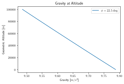
From launch site latitude \(\phi\), the normal gravity \(\gamma\) is found on the ellipsoidal surface (Somigliana’s formula): 1 (pp. 4-1)

\[ \gamma = \gamma_e \cdot \frac{1 + k \sin^2 \phi}{\sqrt{1 - e^2 \sin^2 \phi}} \]

Then, \(\gamma\) is used to find normal gravity \(\gamma_h\) at a geometric height \(h_G\) above the ellipsoid: 1 (pp. 4-3)

\[ \gamma_h = \gamma \cdot \bigg[ 1 - \frac{2}{a} \left( 1 + f + m - 2f \sin^2 \phi \right) h_G + \frac{3}{a^2} h_G^2 \bigg] \]

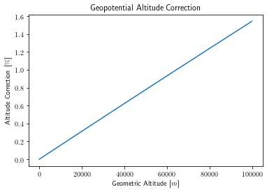
The local geocentric radius of earth is found using the geometry of the ellipsoid: 2

\[ r_e = \sqrt{\frac{(a^2 \cos\phi)^2 + (b^2\sin\phi)^2}{(a\cos\phi)^2 + (b\sin\phi)^2}} \]

This allows the geopotential altitude to be determined: 3 (pp. 8)

\[ h = \frac{r_e \cdot h_G}{r_e + h_G} \]

The difference between geometric and geopotential altitude is nonzero, but does not become significant until high altitudes; for example, at a geometric altitude of 65 km the geopotential altitude is ~1% less.

Constant(s)		Value	Units
\(\gamma_e\)	Normal gravity at the equator (on the ellispoid)	9.7803253359	\(\frac{m}{s^2}\)
\(k\)	Somigliana’s Formula - normal gravity formula constant	1.931852652458e-3	-
\(e\)	First eccentricity of the ellispoid	8.1819190842622e-2	-
\(a\)	Semi-major axis of the ellipsoid	6378137.0	\(m\)
\(b\)	Semi-minor axis of the ellipsoid	6356752.3142	\(m\)
\(f\)	WGS 84 flattening (reduced)	3.3528106647475e-03	-
\(m\)	Normal gravity formula constant (\(\frac{\omega^2 a^2 b}{GM}\))	3.449786506841e-3	-

Atmosphere Model

Input(s)		Units		Output(s)		Units
\(h\)	Geopotential altitude (MSL)	\(m\)		\(T\)	Temperature	\(K\)
\(g_0\)	Gravity at sea level	\(\frac{m}{s^2}\)		\(p\)	Pressure	\(Pa\)
\(T_0\)	Launch site ambient temperature	\(K\)		\(\rho\)	Density	\(\frac{kg}{m^3}\)
\(p_0\)	Launch site ambient pressure	\(Pa\)		\(a\)	Speed of sound	\(\frac{m}{s}\)
				\(\mu\)	Dynamic viscosity	\(\frac{kg}{m \cdot s}\)

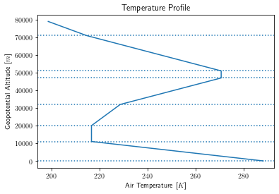
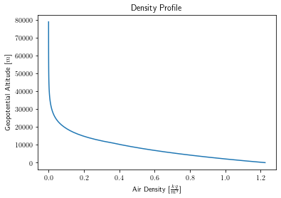
The US Standard Atmosphere 1976 3 is used to determine the atmospheric quantities at a given altitude.

The temperature gradient (also known as “lapse rate”) is given across several altitude regions: 3 (pp. 3)

Geopotential Altitude [\(km\)]	Temperature Gradient [\(\frac{K}{km}\)]
0	-6.5
11	0.0
20	+1.0
32	+2.8
47	0.0
51	-2.8
71	-2.0
84.8520	n/a

The ambient temperature at a given altitude can be found with a simple linear relationship: 3 (pp. 10)

\[ T = T_1 + \frac{dT}{dh} (h - h_1) \]

where \(T_1\) is the temperature at the previous region boundary.

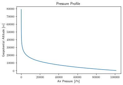
The pressure profile for an isothermal region (\(\frac{dT}{dh} = 0\)) is: 4 (pp. 75)

\[ p = p_1 \cdot e^{-(g_0/RT)(h-h_1)} \]

While the pressure profile for a gradient region (\(\frac{dT}{dh} \neq 0\)) is found by: 4 (pp. 76)

\[ p = p_1 \cdot \left( \frac{T}{T_1} \right)^{-g_0/(\frac{dT}{dh}R)} \]

Again, where \(p_1\) is the pressure at the previous region boundary. To initialize this model, an initial temperature \(T_0\) and pressure \(p_0\) at ground level is propagated upwards to generate the values at each boundary.

With temperature and pressure known, the density at altitude is simply found from the equation of state for a perfect gas: 4 (pp. 58)

\[ p = \rho R T \quad\Rightarrow\quad \rho = \frac{p}{RT} \]

The speed of sound \(a\) is given as a function of temperature: 4 (pp. 107)

\[ a = \sqrt{\gamma \cdot R \cdot T} \]

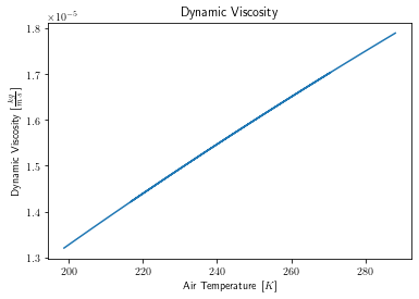
Finally, Sutherland’s Law 5 is used to determine the dynamic viscosity of air \(\mu\):

\[ \mu = \mu_{ref} \left( \frac{T}{T_{ref}} \right)^{3/2} \frac{T_{ref} + S}{T + S} \]

Constant(s)		Value	Units
\(R\)	Specific gas constant of air	287.053	[\(\frac{J}{kg \cdot K}\)]
\(\gamma\)	Specific heat ratio of air	1.40	-
\(T_{ref}\)	Reference temperature	273.15	[\(K\)]
\(\mu_{ref}\)	Viscosity of air at \(T_{ref}\)	1.716e-5	[\(\frac{kg}{m \cdot s}\)]
S	Sutherland constant	110.4	[\(K\)]

References

---

1(1,2,3)

National Geospatial-Intelligence Agency (NGA). (2014). Department of Defense World Geodetic System 1984. https://earth-info.nga.mil/php/download.php?file=coord-wgs84

2

Geocentric radius. (2022, February 10). In Wikipedia. https://en.wikipedia.org/wiki/Earth_radius#Geocentric_radius

3(1,2,3,4)

National Oceanic & Atmospheric Administration (NOAA). (1976). U.S. Standard Atmosphere, 1976. https://www.ngdc.noaa.gov/stp/space-weather/online-publications/miscellaneous/us-standard-atmosphere-1976/us-standard-atmosphere_st76-1562_noaa.pdf

4(1,2,3,4)

Anderson, J. D. (1989). Introduction to Flight (3rd ed.). McGraw-Hill.

5

Sutherland’s law. (2008, October 25). CFD Online. Retrieved February 10, 2022, from https://www.cfd-online.com/Wiki/Sutherland%27s_law